Bounding Boxes & Bounding Ellipsoids
Introduction
Bounding geometries for a set of points can be very useful in fields such as robotics and autonomous vehicles. They can also be applied to some niche fields such as geometrically bounding covariance matrices.1 They can be difficult to create, that is, unless you know a few tricks.
Overview
The majority of the bounding box creation methodology presented here was originally defined by Sai Sharath Kakubal in his article “2D Oriented bounding boxes made simple”.2 For consistencies sake, a full walkthrough of this process will be shown in this article as well. The steps of this process are as follows:
- Obtain Sample Data
- Principal Component Analysis
- Rotate the Data to be Axis-Aligned
- Form Axis-Aligned Bounding Box & Axis-Aligned Bounding Ellipse
- Form Oriented Bounding Box & Oriented Bounding Ellipse
Step 1: Obtain Sample Data
The first step to this process is obtaining sample data. In application, this may be obtained in various ways. The data may be point clouds or sampled ellipses, but for our example here we will generate random points to act as our sampled data. Arbitrary biases and standard deviations were added to the data to make it more realistic to actual applications. The data was also rotated to ensure the data was not naturally axis-aligned. 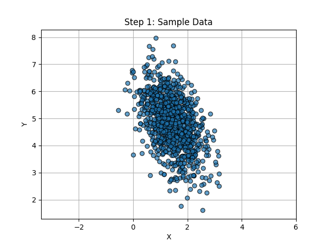
1
2
3
4
5
6
7
8
9
10
11
12
13
14
15
import numpy as np
import matplotlib.pyplot as plt

# generate random points
n = 1000
mean = [3,4]
sigma = [0.5, 1]
data = np.random.normal(loc=mean, scale=sigma, size=(n,2))
data = data.T

# rotate points
theta = np.deg2rad(20)
R = np.array([[np.cos(theta), -np.sin(theta)],
[np.sin(theta), np.cos(theta)]])
rot_data = R @ data
Step 2: Principal Component Analysis
“Principal component analysis, or PCA, reduces the number of dimensions in large datasets to principal components that retain most of the original information.”3 For our purposes, this will be done through calculating the covariance of the sample data and decomposing it into eigenvalues and eigenvectors. The eigenvalues tell you about the spread of the data, while the eigenvectors provide the rotation of the data.
1
2
3
# principal component analysis
P = np.cov(rot_data)
D, V = np.linalg.eig(P) # D is the eigenvalues, V is the eigenvectors
Step 3: Rotate the Data to be Axis-Aligned
To axis-align the data, we first need to center it about the origin. This is accomplished by taking the mean of the data and subtracting it out. Now, utilizing the eigenvector matrix obtained through PCA, the centered data can be rotated to be axis-aligned. 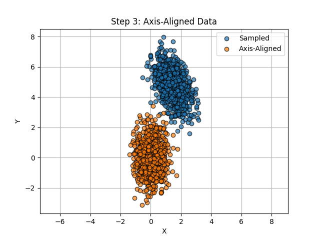
1
2
3
4
# axis-align data
mu = np.mean(rot_data, axis=1)
centered_data = np.transpose(rot_data.T - mu)
aa_points = V.T @ centered_data
Step 4: Form Axis-Aligned Bounding Box & Axis-Aligned Bounding Ellipse
With the data axis-aligned, it is trivial to form a bounding box around it. This is done by finding the maximum and minimum x and y values of the data. These are then subtracted to get the size of the box; i.e. width and height. Using these values, the corner points of the bounding box can be formed. Forming the axis-aligned bounding ellipse (AABE) is a little more tricky. To do this, we have to understand the relationship between the dimensions of the ellipse and the eigenvalues of it’s matrix representation. The matrix form of an ellipse is shown below:
\[xPx^T = c\]Here, \(P\) is the matrix representation of an ellipse. The dimensions of this ellipse are determined by the eigenvalues of the matrix \(P\). This relationship is shown below:
\[d_i = \frac{1}{\sqrt{\lambda_i}}\]where \(d_i\) is the \(i^{th}\) dimension and \(\lambda_i\) is the \(i^{th}\) eigenvalue of \(P\). Given these two relationships, we can calculate the eigenvalues of the bounding ellipse from the following equation:
\[\lambda_i = \left(\frac{\sqrt{2 + 2\nu}}{d_i}\right)^{2}\]where \(\nu\) is a tolerance parameter between 0 and 1. A value of zero means the ellipse fully encloses the bounding box, and a value of 1 means the bounding box fully encloses the ellipse. 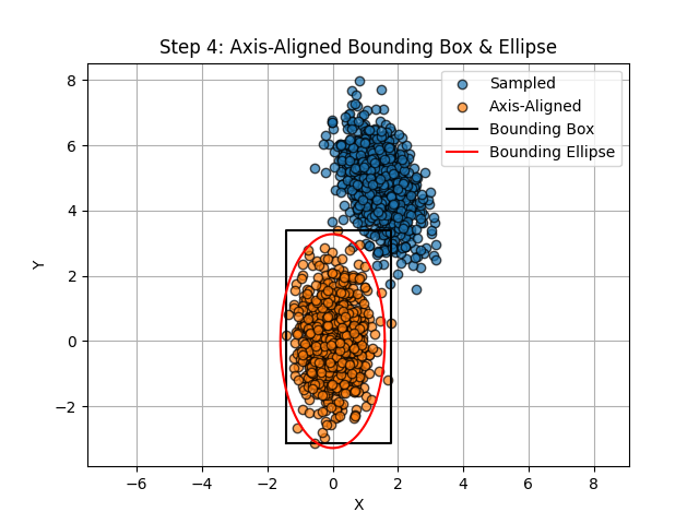
1
2
3
4
5
6
7
8
9
10
11
12
13
# axis-aligned bounding box
mx = np.max(aa_points, axis=1)
mn = np.min(aa_points, axis=1)
sz = mx - mn
x = np.array([mn[0], (mn[0] + sz[0])])
y = np.array([mn[1], (mn[1] + sz[1])])
pts = np.array([[x[0], x[1], x[1], x[0], x[0]],
				[y[0], y[0], y[1], y[1], y[0]]])

# axis-aligned bounding ellipse
tolerance = 1
eigenvalues = ((np.sqrt(2 + (tolerance*2))/(sz))**2)
S_aabe = np.diag(eigenvalues)
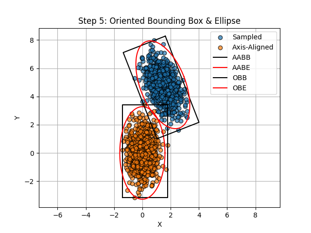
Step 5: Form Oriented Bounding Box & Oriented Bounding Ellipse
Converting the axis-aligned bounding box (AABB) to an oriented bounding box is very simple. The corner points calculated in Step 3 need to be rotated back to the original frame using the eigenvectors obtained through PCA in Step 2. The same thing is done to the axis-aligned ellipse; rotating the new eigenvalues matrix with the eigenvectors calculated in Step 2.
1
2
3
4
5
6
7
# oriented bounding box
obb_pts = V @ pts
obb_pts = np.transpose(obb_pts.T + mu)

# oriented bounding ellipse
tolerance = 1
S_obe = V @ np.diag(eigenvalues) @ V.T
Applications
For my personal research, these bounding geometries were used to geometrically define the innovation covariance of a Kalman filter. This was done by sampling the points for the state and measurement error ellipses, and performing the above calculations to create a bounding ellipse(or in my case ellipsoid) around these error ellipses in order to form a better innovation covariance than the typical Kalman filtering equations. My paper on the topic is “Pedestrian Attitude Estimation using a Multiplicative Extended Kalman Filter with Geometrically-Defined Innovation Covariance”1.
References
Livingston, W. B., & Bevly, D. M. (2025). Pedestrian Attitude Estimation using a Multiplicative Extended Kalman Filter with Geometrically-Defined Innovation Covariance. In 2025 IEEE/ION Position, Location and Navigation Symposium (PLANS) (pp. 1-8). ↩︎ ↩︎2
2D oriented bounding boxes made simple. Scratchpad. (2021, April 20). ↩︎
Ibm. (2025, April 16). What is Principal Component Analysis (PCA)?. IBM. ↩︎